There are many situations that we will need to forecast something in business, either the demand or sales, supply or inventory. Fortunately, we have many tools that have made it easy to generate decent forecast very quickly. R has several packages that provide automated forecasting with a couple lines of code needed. In this post, I will use a store item sales data set from Kaggle to demonstrate the power of four different R packages and six different models to create sales forecast. I will compare the forecasts with the actual values & measure the forecast accuracy. The method with the smallest difference between forecast and actual will be the winner.
The Data
The data I am using is 5 years of daily store-item sales data from multiple stores. It can be downloaded from Kaggle here. The data ranges from year 2013 to 2017. We will summarize it into monthly total sales data, use the Jan 2013 to June 2017 data to train the models and July 2017 to Dec 2017 six months of data as hold out period to compare the models.
We first load the data, aggregate the sales from all stores by month, plot the data to examine the patterns and then divide the data set into training and test.
library(tidyverse)
library(lubridate)
#read in the data
df=read.csv("~/your directory/demand-forecasting-kernels-only/train.csv")
df$date = as.Date(df$date)

df_sales <- df %>%
  mutate(ds=floor_date(date, unit="month")) %>%
  group_by(ds) %>%
  summarize(y = sum(sales))
plot(y ~ ds, df_sales, type = "l", main="Monthly Total Sales")
train<-df_sales[1:54,]
test<-df_sales[55:60,]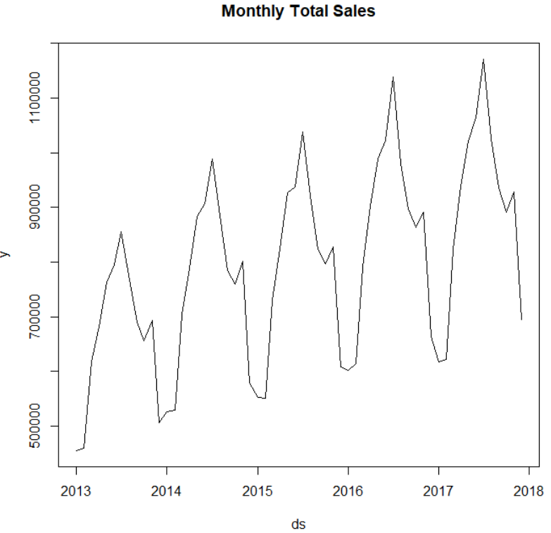
The Packages and Models
The four R packages we use are prophet, fable, forecast and RemixAutoML packages.
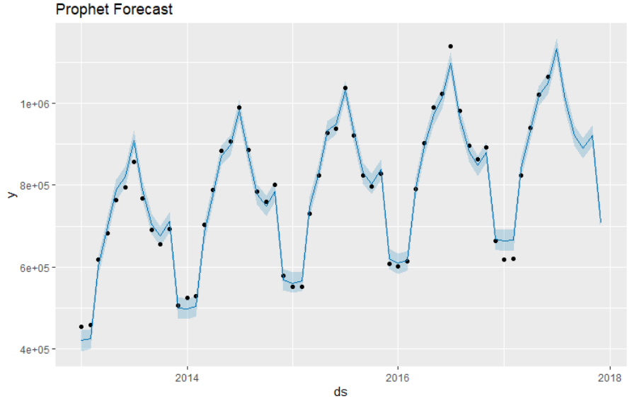
Prophet is able to produce reliable and robust forecasts (often performing better than other common forecasting techniques) with very little manual effort while allowing for the application of domain knowledge via parameters.
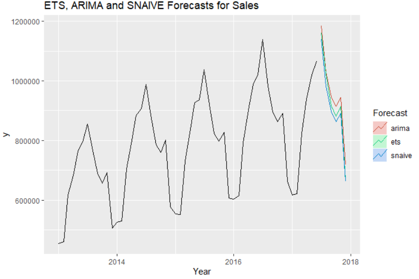
The fable package is designed to work with tsibble data and can handle many time series. It is part of the tidyverts family of packages for analyzing, modelling and forecasting many related time series. We will demonstrate its use on this single time series. For this data set, a reasonable benchmark forecast method is the seasonal naive method (snaive), where forecasts are set to be equal to the last observed value from the same quarter. Alternative models we fit for this series are ETS (exponential smoothing state space model) and the ARIMA model.
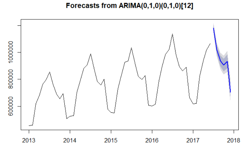
The forecast package’s auto.arima() function returns the best ARIMA model based on performance metrics. It is almost always better to use the auto.arima() function than calling the arima() function directly. We will see it from this example soon.
AutoTS() function in RemixAutoML package is also very easy to use. AutoTS stands for automated time series, and it automatically finds and creates the most accurate forecast from a list of 7 econometric time series models including ARIMA, Holt-Winters, and Autoregressive Neural Networks.
We can call all these functions to perform the forecasts with only a few lines of code each.
######## prophet model #######
library(prophet)
m<-prophet(train)
future <- data.frame(ds=df_sales$ds)
forecast_prophet <- predict(m, future)
plot(m, forecast_prophet) +  ggtitle("Prophet Forecasat")

####### forecast with fable ######
library(fable)
library(tsibble)

train_tsbl <- train %>%
  mutate(month = yearmonth(ds)) %>%
  as_tsibble(index=month)

fit <- train_tsbl %>%
  model(
    snaive = SNAIVE(y ~ lag("year")),
    ets = ETS(y),
    arima = ARIMA(y)
  )

# forecasting
forecast_fable = forecast(fit,h=6)

forecast_fable %>%
  autoplot(train_tsbl, level = NULL) +
  ggtitle("Forecasts for Sales") +
  xlab("Year") +
  guides(colour = guide_legend(title = "Forecast"))

######## ARIMA ########
library(forecast)
ts_train = ts(train$y, start=2013, frequency=12)
AutoArimaModel=auto.arima(ts_train)
forecast_autoarima = forecast(AutoArimaModel,h=6)
plot(forecast_autoarima)

########## Forecast with autoTS #############3
library(RemixAutoML)
output <-   AutoTS(data=train,
                   TargetName= "y",
                   DateName = "ds",
                   FCPeriods= 6,
                   HoldOutPeriods= 3,
                   TimeUnit= "month")
forecast_autots <- output$Forecast
The plots give us a good idea of how each model forecasts on the later half of 2017.
Model Comparisons
From the plots, we see that all forecasts look pretty reasonable. We need a way to decide which method is the best for this data set. We will need to calculate the errors between forecast and actual and whichever has the smallest error is the champion model.
There are many ways to calculate errors between forecast and actual. The two standard errors are mean absolute error (MAE) and Root Mean Squared Error(RMSE). The first one is to calculate the absolute difference between the forecast and the actual value from July to December and then average the absolute errors to get the mean absolute error.
The second standard error metric is one I prefer because it penalizes large differences which do not show up in the Average error. To penalize large errors, one gets the square of each months error and adds them for the three months and get the average. The square root of that value is the error that captures large errors and is called Root Mean Squared Error (RMSE)
There is also one more error that is popular which is Mean Absolute Percentage Error (MAPE) where the error is a percentage.
Though all 3 are valid ways to measure the error, I will use RMSE to compare models next as it penalizes large deviations from the actual value.
######## compare forecast accuracy among models with rmse ########
library(mltools)

forecast_autots_model <-forecast_autots %>% select(2) %>% unlist()

for (modelname in c('snaive', 'ets','arima','prophet', 'autots', 'autoarima')){
  cat('model ', modelname, '\n')
  if (modelname == 'autots') {cat('RMSE ', rmse(forecast_autots_model, test$y),'\n')}
  else if (modelname == 'prophet')
  {cat('RMSE ', rmse(forecast_prophet$yhat[55:60], test$y), '\n')}
  else if (modelname == 'autoarima')
  {cat('RMSE ', rmse(forecast_autoarima$mean, test$y), '\n')}
  else {cat('RMSE', rmse(forecast_fable$y[which(forecast_fable$.model == modelname)], test$y) , '\n')}
}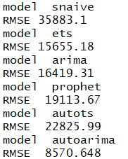
The auto.arima() model has the lowest RMSE. Thus it is the most accurate in forecasting on our hold out period among all the models we tried for this data set. It is selected as the winner.
Summary
The purpose of this post is to show you some quick and easy ways to come up with good forecasts. If more precision is needed, we will need more tuning or add more information into the model to help predict the outcome. For example, when predicting the number of sales or number of calls to the call center, those forecasts correlate to inventory and human resources investment to react to the forecast. So when there is an action to be taken that costs $$$, we probably want to go with an approach that has better precision. I will cover this in a future post.